Creating a question

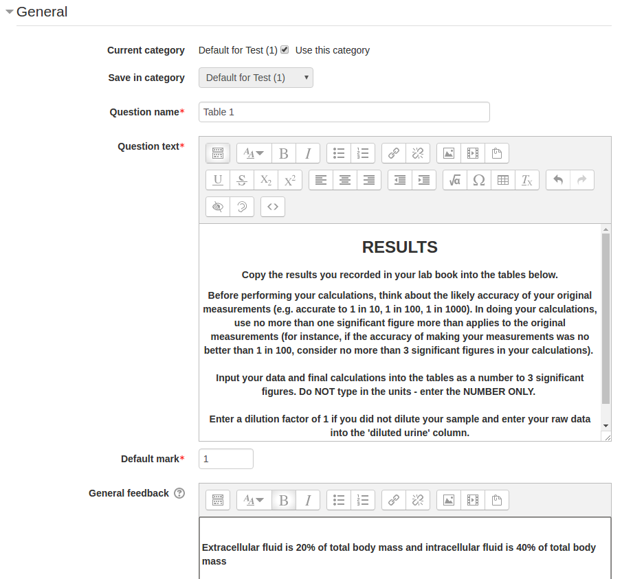
When setting up the question, the first part looks familiar as a Moodle question with places to enter a question name, question text and general feedback:

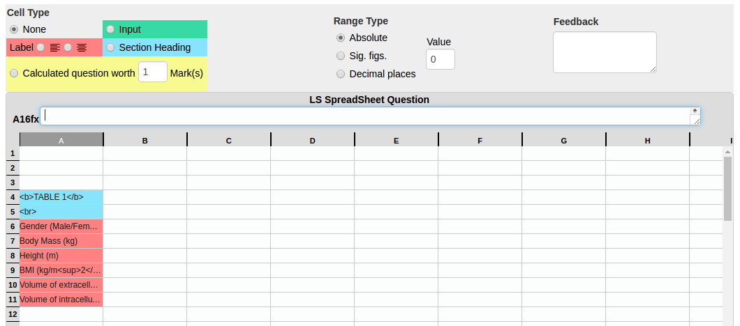
Underneath this is a spreadsheet where you will set up a table containing column, row headings and cells for students to enter data and their calculations:

---

1. Start by entering a title for your table (if there will be one) and the column and row headings.

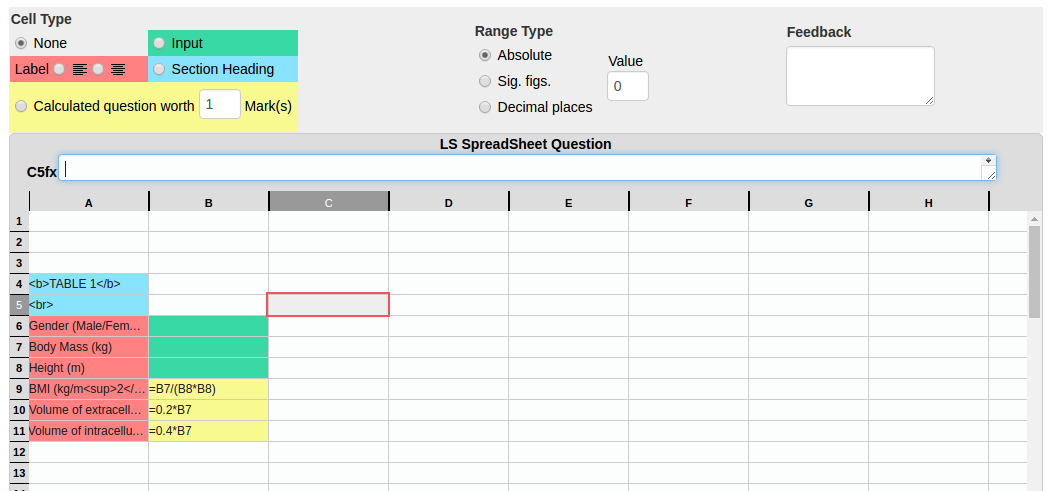
Unlike Excel, you are not able to insert rows or columns so you may wish to leave a few blank rows above (and possibly a couple of columns to the left of) the table in case you need to move cells around later on. Remember to leave a blank row wherever you want space between the title and table or different parts of the table.

2. Format the column and row headings using the radio buttons on the top left of the spreadsheet.

A section heading (blue) means that this will take the whole row and is used for titles or breaks in a table.

A label (pink) may be left aligned or centre aligned. This is a heading within a table and does not take up the whole row. Usually, left aligned labels are used for row headings and centre aligned row headings for column headings.

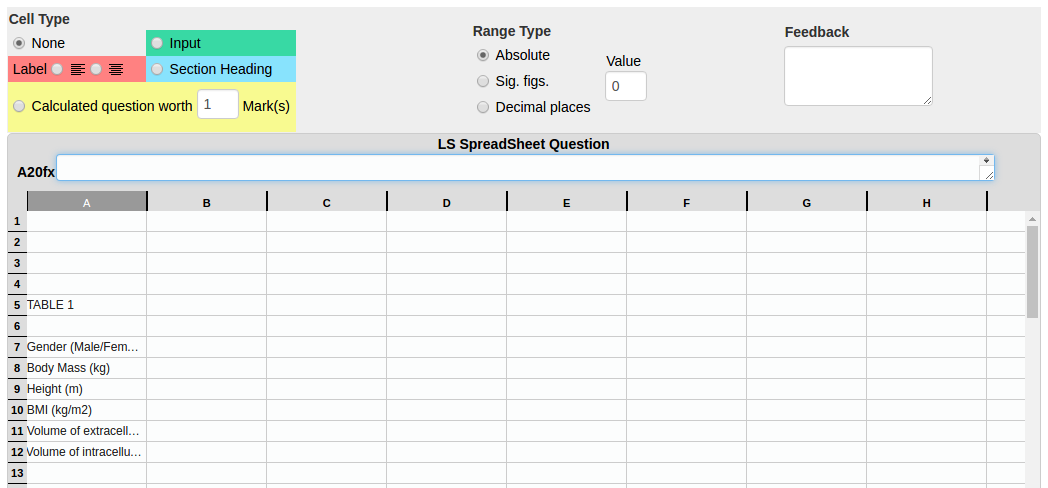
Anything that is not formatted using the radio buttons will be ignored and not appear when you preview the question.

3. Format any text in the column and row headings using html tags.

You will need both an opening and a closing tag. These should be placed at the start and end of the text to be formatted.

Example tags:

<b>Your text</b>		bold
<i>Your text</i>		italics
<u>Your text</u>		underline
<sup>Your text</sup>	superscript
<sub>Your text</sub>	subscript

Line breaks can be added using the
tag (no closing tag is required) and this needs to be formatted as a section heading (blue).

4. Format any cells where students should enter unmarked data using the input radio button.

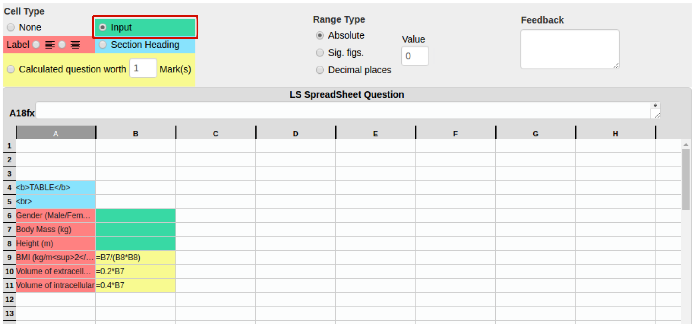
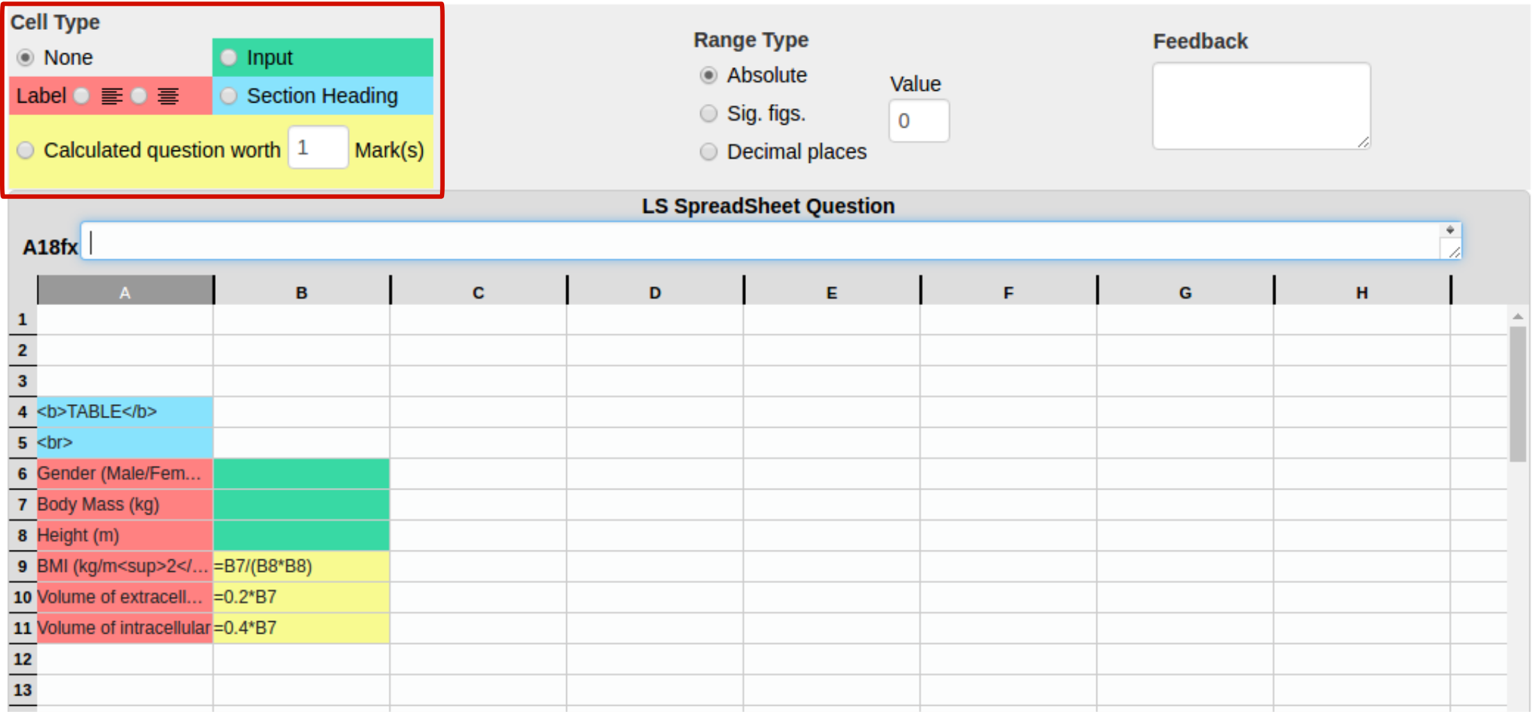
5. Enter the formulae for the answers to any calculations students should perform (or stages of these calculations) using the standard Excel format.

Note that unlike Excel you will have to type in the cell references and cannot enter them by simply clicking on the appropriate cell in the spreadsheet. All simple functions will work in the spreadsheet question but be wary when using more complex functions, such as those for statistical tests, as not all formulae will work.

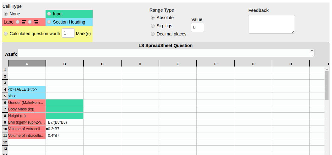
6. Format any cells where students should enter calculated values using the calculated question radio button.

When formatting cells as calculated questions, you will also need to set how many marks are available for each calculation. The default is 1 mark per cell but you can change this on a cell to cell basis.

7. Set the range for each cell formatted as a calculated question.

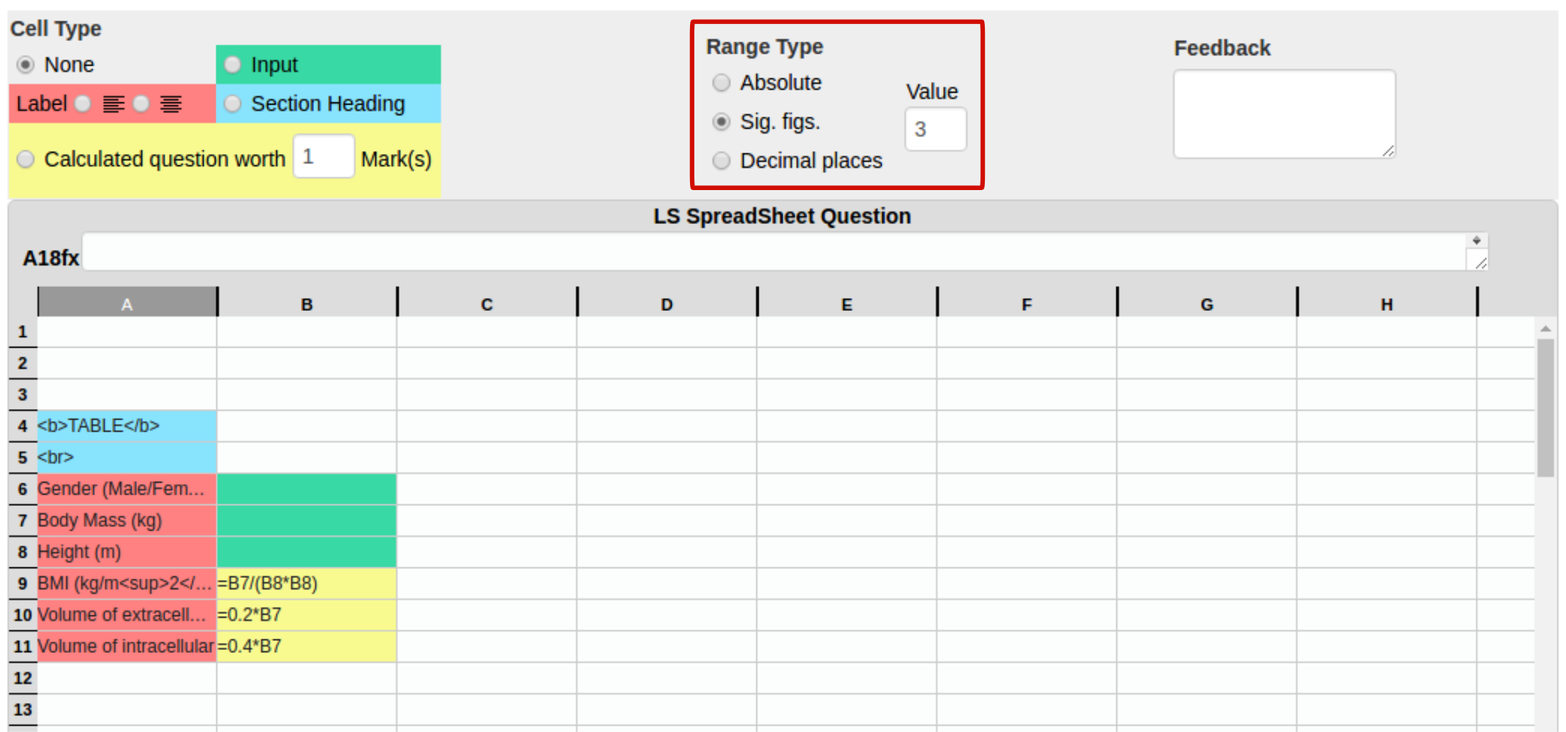
Select a cell and then use the area indicated above the spreadsheet to set whether the question should be marked according to the number of decimal places, significant figures or whether an absolute range should be used.

Enter the number of decimal places or significant figures into the value box to the left of these radio buttons. In this example, the calculation will be marked as correct to 3 significant figures.

Absolute range

Using an absolute range will mean the calculation will be marked as correct if it is the expected figure plus or minus whatever is entered into the value box.

For example, if the expected answer based on a student’s raw data was 20.414573 and the range was set as absolute with 2 entered into the value box, anything between 18.414573 and 22.414573 would be marked as correct.

Significant figures

Using the significant figures option will mean that a calculation is marked as correct if the correct answer is provided to at least this many significant figures.

For example, if the absolute answer is 20.414573 and the question is marked to 3 significant figures:

• 20 would be marked as incorrect
• 20.4 would be marked as correct
• 20.41 and anything with more decimal places than this would also be marked as correct

Decimal places

Using the decimal places option will mean that a calculation is marked as correct if the correct answer is provided to at least one decimal place. However, the numbers after the decimal point can be anything and are not marked. For this reason, it is advisable to use significant figures and not decimal places.

For example, if the absolute answer is 20.414573 and the question is marked to 3 decimal places:

• 20 would be marked as incorrect
• 20.4 would be marked as correct
• 20 followed by a decimal point and any other numbers would also be marked as correct

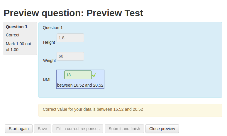
Whichever option is selected, feedback as to the correct answer or the range of correct answers is automatically provided when you have submitted the question and roll over a calculated question.

In this example, the correct answer is 18.52 and an absolute range of 2 has been set:

8. Enter specific feedback for each calculation (if required).

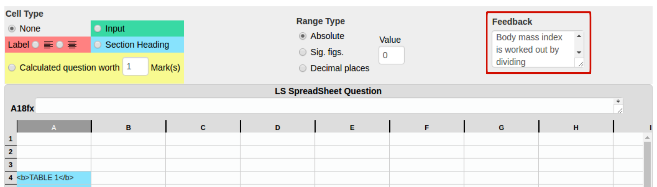
As well as the general feedback that will appear beneath the question (in the same way as many other Moodle questions), you can also provide feedback specific for each calculation. This can only be plain text (no formatting) and cannot include images. It is entered by selecting the appropriate cell and then typing the feedback into the box indicated above the spreadsheet. You can expand this box by dragging the bottom left hand corner.

This type of feedback will appear when reviewing a quiz by rolling over the relevant cell or cells. If using calculation specific feedback (as opposed to just the general feedback), it is a good idea to use the general feedback box to instruct students to rollover the calculations for feedback as this may not be intrinsically obvious.

Testing the question

Once you have completed the question, save it for a final time (you should have been saving it throughout the setup process anyway) and preview it. If anything looks odd, go back to edit the question and rectify the problem.

The button on the top right of the spreadsheet can be used to flick between editing view (showing the formulae) and calculated view (showing data). The calculated view allows you to enter raw data and see what the correct answers would be for this raw data so you can check the question is working as expected. You may need to flick between editing and calculated view to see the correct answers.

Common issues

Change to a cell not visible

Note that once you have made a change to a cell, you may have to click elsewhere in the spreadsheet before saving to see this change take effect.

Issue with changing formatting (colour) of cell

You may find that sometimes when changing the formatting (colour) of a cell, it won’t change away from the existing formatting. If this happens, try clicking elsewhere in the spreadsheet. If this doesn’t help, try setting the formatting to none, clicking elsewhere in the spreadsheet, saving the question and reopening it before setting it to the correct formatting.

Sometimes, when changing the formatting of a cell or a group of cells, the cell that was highlighted previously also changes formatting. If this happens, you will need to reset the formatting for this cell.

Decisions

There is a 2% leeway on any correct answer. This is to allow for different intermediate roundings in multiple step calculations (getting the calculation essentially right but multiple roundings shifting the “correct” value.

Set =ROUNDSIGFIG((B2/6220*1e6),3) which sets the value which is being evaluated against the correct number of sig figs.