Home
Setting Up and Reviewing Analyses with the Archive Walker GUI
Archive Walker (AW) is a tool designed to ingest, analyze, and visualize PMU data and the power system events that can be found within it. It is open source, with development funded by Bonneville Power Administration (BPA) and the US Department of Energy (DOE). The goal of AW is to bring value to archives of PMU data by enabling analysis with a set of built in event detectors and reducing the overhead required to prototype and deploy new analysis methods.
The AW tool is compatible with the Windows operating system. It is composed of two components: an underlying MATLAB engine and a user interface written in the .NET framework. These components rely on the MATLAB runtime and the .NET framework, both of which can be downloaded for free. First, download .NET framework 4.6.1 at https://www.microsoft.com/en-US/download/details.aspx?id=49982. Next, download the R2018a (9.4) MATLAB runtime at https://www.mathworks.com/products/compiler/matlab-runtime.html. Finally, transfer the executables downloaded from these links to the computer that will host AW and run them to install the .NET framework and MATLAB runtime.
Next, AW can be downloaded as a zip file at https://github.com/pnnl/archive_walker/releases. Once downloaded, unzip the file by right clicking on it. The resulting folder contains the following subfolders: ArchiveWalker, ArchiveWalkerRealTimeDisplay, and openHistorianPresetWriter. The main Archive Walker tool is contained in the ArchiveWalker folder. The majority of this documentation is dedicated to its use. The Real-Time Display and openHistorian Preset Writer applications are described in the Companion Tools Section.
To launch AW, simply double click the ArchiveWalker.exe file located within the ArchiveWalker folder. There will be a brief delay the first time the tool is launched.
Examples of the GUI’s layout are presented in Figures 1-4. The Project panel on the left side of the screens will be discussed in the Project Panel Section. The Signal Selection panel visible on the right side of the screen when the Settings page is selected will be described in Signal Selection Panel Section. The Data Sources Tab Section through the Detection Tab Section discuss the Settings tabs used to configure AW, and the Reviewing Results Section covers how to review results under the Results page.
The discussion in the Reviewing Results Section utilizes the preloaded example data and results included in the download of AW. These examples cover each of the detectors. The data is stored in the ExampleData folder and the results are stored in the Projects folder. To access these examples, ensure that the specified results storage location is the Projects folder (see the Project Panel Section for instructions). When the GUI is opened for the first time, the results path defaults to this folder.
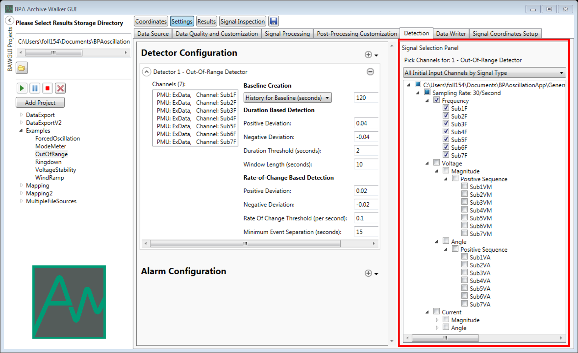 Figure 1: Example GUI layout with Settings page selected.
 Figure 2: Example GUI layout with Results page selected.
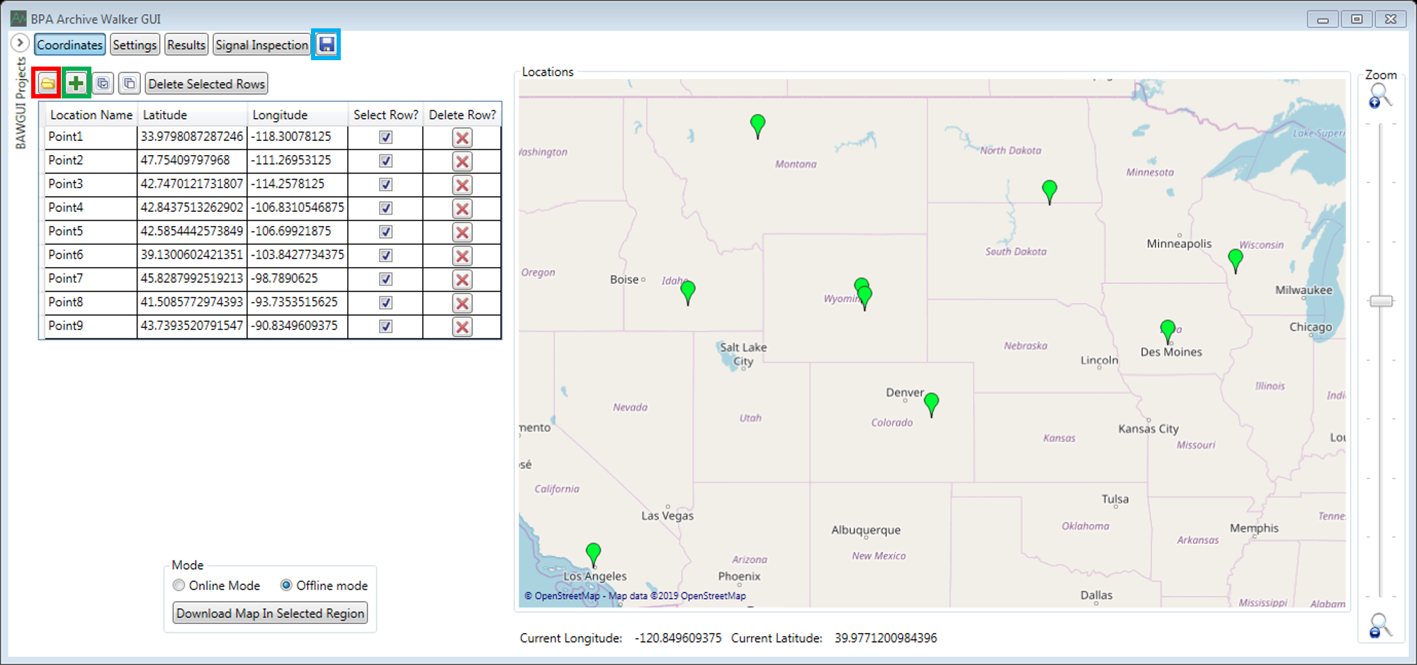 Figure 3: Example GUI layout with Coordinates page selected.
 Figure 4: Example GUI layout with Signal Inspection page selected.
The final step in preparing to use AW is choosing where results should be stored. AW was designed to allow detailed review of detection results while minimizing required disk space. Still, analyses of large archives may require significant storage. The amount of storage required is dependent on factors such as the number of PMUs in the dataset, the sampling rate, and the number of preprocessing steps, but it is on the order of one GB for each day of data. The Projects folder mentioned earlier in this section serves as the storage location for results the first time AW is opened. If this is undesirable, create a new folder where you would like results to be stored. The path to this folder will be entered in the GUI before beginning analysis.
The panel along the left side of the GUI (see the red box in Figure 5) allows the user to set up projects and specify where results should be stored. The path at the top of the panel specifies where results will be stored. Clicking the folder button below the path allows the user to select a different path for results. The first time AW is opened, the Projects folder included in the zip file is selected as the results storage location. This folder contains examples that are described in Examples Section.
 Figure 5: Project panel (left) and Settings page (right).
Results are organized into projects and tasks. A task is comprised of a set of results associated with a specific analysis setup. Tasks are stored within projects for organizational clarity. After a project is added by clicking the “Add Project” button, tasks can be created by right clicking on the project name (see the green box in Figure 5). Right clicking also allows the entire project to be deleted. New tasks are also created when the save button is clicked after the setup of an existing task is altered.
Once the setup for a task is complete, it can be applied to data by clicking the play button (green arrow). While a task is running, a green arrow appears next to the task name. The remaining buttons allow a task to be paused/resumed, stopped, or deleted.
The panel on the right side of the GUI, indicated by the red box in Figure 1, is used to select signals when setting up analyses. The dropdown at the top of the panel provides options for how to select signals. The options fall in three categories: 1) Initial set of signals contained in the data, 2) output signals from previous tabs, and 3) inputs and outputs from steps on the current tab. For the first two categories, the signals can be organized by PMU or by signal type. Signals are also organized by their sampling rate because all signals at the input to any step in AW must have the same sampling rate. In the following, the ringdown detector example, which is discussed in more detail in Ringdown Detector Example Section, will be used to illustrate the functionality of the Signal Selection panel.
Examples of the three categories of signal selection are illustrated in Figures 6, 7, and 8. In Figure 6, the first step of the analysis setup is to unwrap voltage angles included in the input data. The data is being organized by signal type, rather than PMU, because only voltage angles are of interest. After unwrapping, a filter is applied to the signals before passing them into a multirate step. When the same set of signals is desired for multiple steps, it is convenient to use the Output Channels by Step option in the dropdown, as in Figure 7. In the figure, the inputs to multirate processing can be selected easily by clicking either the Step 1 or Step 2 checkboxes (note that the signals are identical). After signal processing, the signals are ready to be passed to the ringdown detector. In Figure 8, these signals are selected by displaying outputs from the Signal Processing tab. At each step, the functionality of the Signal Selection tab makes it easier to locate the signals of interest, making it significantly easier to configure AW. Details on the setup process are provided in the following sections.
 Figure 6: Selecting voltage angle signals to be unwrapped from the input data using the Signal Selection panel.
 Figure 7: Selecting signals from previous steps for input to the multirate processor using the Signal Selection panel.
 Figure 8: Selecting signals from the Signal Processing tab for analysis with the ringdown detector using the Signal Selection panel.
This page allows the user to specify the geographic locations where signals originate. The page is depicted in Figure 3. The locations can be assigned to signals under analysis on the Signal Coordinates Setup Tab. To add a new location, left-click on the desired location on the map and enter the location's name. Alternatively, a new row can be added to the table by clicking the green + button (highlighted by a green box in Figure 3). The map can be zoomed in and out using the mouse's scroll button or the slider on the right side of the screen. To pan, hold the right mouse button and drag.
Locations are stored within the SiteCoordinatesConfig.xml file, which AW saves to the results storage folder specified at the top of the Project Panel. To load a SiteCoordinatesConfig.xml file from a different location, click the folder button (highlighted by a red box in Figure 3). Clicking the save button (highlighted by a blue box in Figure 3) will then replace the current file.
This page, which is depicted in Figure 4, allows the user to plot signals read, produced, and analyzed by AW. It is typically reached from the File Sources Panel or a results tab (see these sections for additional information on the page's use).
Once signals have been loaded, they will appear in the Signal Selection Panel. To add a plot, click the Add a Plot button highlighted by a red box in Figure 4. Plots can be collapsed using the arrow button highlighted by a green box in Figure 4. Once a plot is expanded, add signals to the plot by selecting them from the Signal Selection Panel. To automatically adjust scaling, press the a key while a plot is selected. To export data from a plot, right-click and select the Export Data option.
To conduct spectral analysis, right click on a plot and select the Spectral Inspection option. A Welch Periodogram will be applied to each signal and the result will be displayed on a new Spectral Inspection tab, as in Figure 4. The parameters for the Welch Periodogram can be adjusted using the fields in the lower right panel, which is highlighted with a blue box in Figure 4. The analyzed data begins at the leftmost sample of the time-domain signal and continues for the number of seconds specified by the Analysis Length field. This data is broken into segments with length specified by the Window Length field and windowed using the type of window specified by the Window dropdown. Each window overlaps the adjacent segment of data by the number of seconds specified in the Window Overlap field. Simple periodograms are calculated at a number of frequency bins specified by the Zero Padding field and then averaged together to form the Welch Periodogram. The Log Scaling checkbox affects the scaling y-axis of the plot, and the Frequency Range fields allow the user to specify the range of x-axis values.
This tab allows the user to specify a set of PMU data for analysis.
The user specifies information about the sources of data. The required information depends on whether the data is stored in files or in a database. This selection is made using the File Type Dropdown described in the File Type Dropdown Section and determines what data is required, as described in the Files as Source and Database as Source sections. Archive Walker can read from multiple sources, even if they have different sampling rates. If data is stored in files, Archive Walker requires that files from different sources cover corresponding time periods, e.g., all files could be one minute in length and start at the top of the minute.
The File Type dropdown allows the user to specify a data source/format. The options available in the dropdown are described in the following subsections.
A custom file type used by the Bonneville Power Administration (BPA) to store synchrophasor measurements.
A generic format for CSV files developed by the Western Electricity Coordinating Council (WECC) Joint Synchronized Information Subcommittee (JSIS). Figure 9 contains the relevant section from the JSIS document “WECC Guideline for Data Format Used in Engineering Analysis Applications of Disturbance and Simulated Data.” The full list of signal types and units compatible with Archive Walker are listed in Table 1.
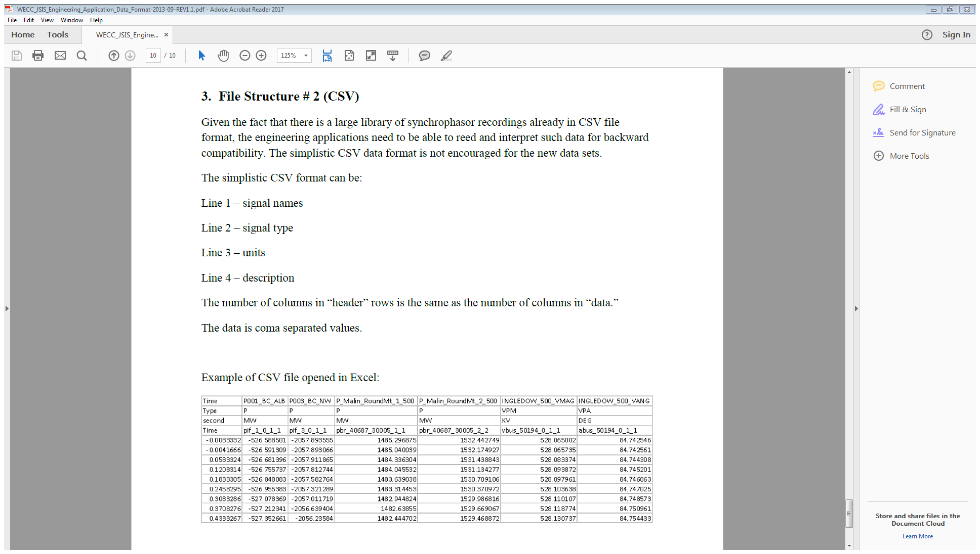 Figure 9: Information on the JSIS-CSV format from the JSIS document “WECC Guideline for Data Format Used in Engineering Analysis Applications of Disturbance and Simulated Data.”
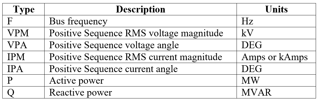
Table 1. List of Signal Types and Units Compatible with Archive Walker.
A custom file type used by the BPA to store synchronized point-on-wave measurements.
A third-party data storage solution used by the electric power industry. See https://www.osisoft.com/pi-system/ for additional information.
A third-party data storage solution used by the electric power industry. See https://github.com/GridProtectionAlliance/openHistorian for additional information.
If the user selects PDAT, JSIS CSV, or HQ Point on Wave from the File Type Dropdown, then AW will uses an example file specified by the user to determine the location and naming convention of the data.
AW must know which signals will be available for analysis, so an example file is required. The path to the example file can be entered into the field manually, or the user can navigate to it using the folder button next to the field (see Figure 5). Once the field is filled, clicking the Read File button will load the PMU and signal names into the GUI for display while setting up analyses. It also automatically fills the File Directory and Mnemonic fields for the user’s review. These fields cannot be edited directly, but their entries are described in the File Directory Field Section and the Mnemonic Field Section to provide additional information about how data should be stored. Clicking the Inspect Signal button loads the file and opens the Signal Inspection Page to allow the user to plot the input signals.
After a task is executed, it cannot be modified without saving it as a new task to prevent results from being destroyed inadvertently. The exception is the example file. As detailed in Transferring the Location of Results and Data Section, the example file can be updated so that data and results can be shared by different users.
Specifies the main folder containing a source of data files. It can have any name, but subfolders must adhere to the following convention. Inside the main folder, PMU data is sorted by timestamp into folders with names corresponding to the four-digit year of the timestamp. Within each year folder, PMU data is sorted by timestamp into folders with names corresponding to the convention YYMMDD, where YY corresponds to the two-digit year, MM corresponds to the two-digit month, and DD corresponds to the two-digit day of the month. Individual data files are stored within the folders specifying the date. For example, with a main folder path of C:\PMUdata, the path to the folder containing data files timestamped at any time on November 2, 2014 would be
C:\PMUdata\2014\141102.
Files are expected to adhere to the following convention:
MNEMONIC_YYYYMMDD_HHMMSS.csv(pdat)
where MNEMONIC is a set of characters excluding underscore, YYYYMMDD specifies the file’s start date, and HHMMSS specifies the file’s start time. The MNEMONIC portion of the name should appear in the Mnemonic field.
If the user selects PI Database or openHistorian from the File Type Dropdown, then AW uses a preset file specified by the user to determine which signals to read from the database. This preset file is generated by either the PI Database Reader tool (https://svn.pnl.gov/FRTool/wiki/PDRManual) or the openHistorian Preset Writer tool. Further details are provided in the following subsections.
AW must know which signals will be available for analysis, so a preset file is required. The path to the preset file can be entered into the field manually, or the user can navigate to it using the folder button next to the field (see Figure 10). Once the user fills the Example File field, AW automatically fills the File Directory field and populates the Preset dropdown.
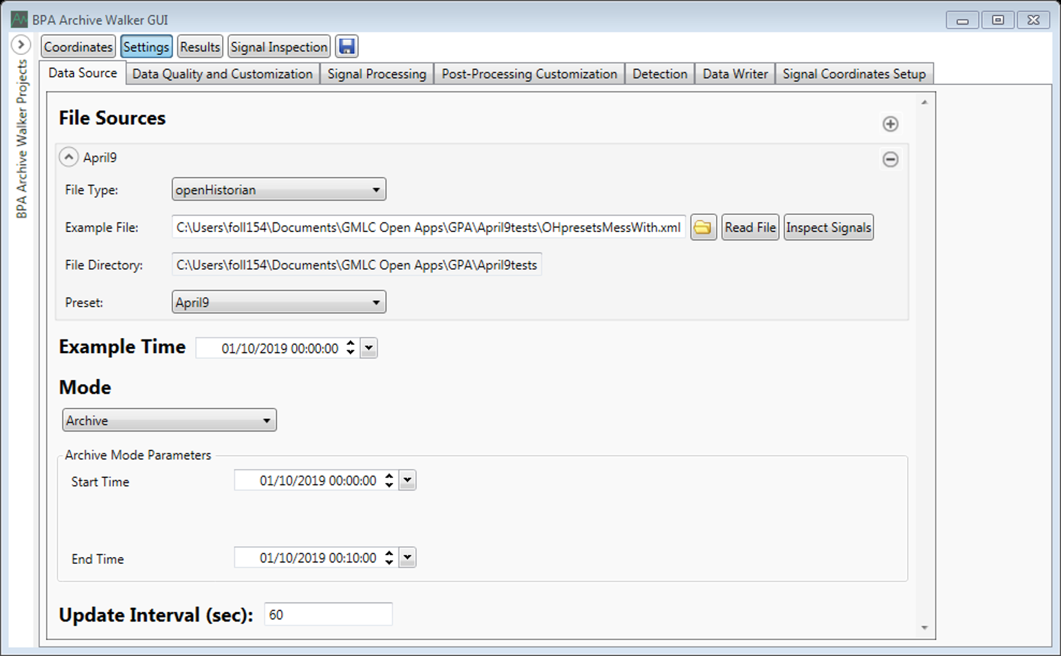 Figure 10: Example File Sources panel when using a database as a data source.
After a task is executed, it cannot be modified without saving it as a new task to prevent results from being destroyed inadvertently. The exception is the example file. As detailed in Transferring the Location of Results and Data Section, the example file can be updated so that data and results can be shared by different users.
The path to the folder containing the example (preset) file.
List of presets specified in the preset file generated by either the PI Database Reader tool or the openHistorian Preset Writer tool. Each preset specifies a set of signals to be read by AW during analysis.
Retrieves the names of signals listed in the preset selected in the Preset Field for display in AW while setting up analyses.
Retrieves the data for signals listed in the preset selected in the Preset Field and opens the Signal Inspection Page to allow the user to plot the input signals. One minute of data is loaded beginning at the time specified in the Example Time field.
Specifies the beginning of the time period to be retrieved when the Inspect Signals button is pressed.
The user specifies which data should be analyzed and how the tool should move through the files.
The user specifies the mode that the tool should operate in.
Runs from a user-specified range of times, immediately skipping over any missed files.
Begins processing from the most recently available file (selected based on computer’s system clock in UTC) and continues to process files as they become available. If a file is missing, the tool will wait a user-specified amount of time for it to be written.
The tool begins in Archive mode before transitioning to Real-Time mode.
In Archive and Hybrid modes, specifies the timestamp of the first file to be processed.
In Archive mode, specifies the timestamp of the last file to be processed.
When Real-Time or Hybrid mode is selected, a set of fields will appear allowing the user to specify how the tool should handle data no longer being available (first sentence) and gaps in the data (second sentence).
When Hybrid mode is selected, a field will appear as part of a sentence to allow the user to specify when the tool should transition from Archive mode to Real-Time mode.
When a database is being used as a data source, this field specifies the length of data that should be analyzed at each step. If data sources are exclusively file based, the update interval does not need to be specified. However, the update interval must be specified regardless of whether files or databases serve as the data source when the forced oscillation detector, voltage stability detector, or mode meter are implemented.
The user specifies which data quality filters should be implemented and how custom signals should be created from the base signals in the data files. Filters and customizations are added by clicking the  dropdown in the upper right corner of the panel.
These filters allow the user to examine signals for data that is missing, corrupt, or otherwise compromised. Later, in the Data Processing tab, the user can specify how to interpolate through periods of bad/missing data.
Filters the data based on status flags stored alongside the data in the processed files. Note that this is the only data quality filter that operates on all signals from a particular PMU, rather than on specific signals. Also note that JSIS-CSV files do not contain status flags.
This filter flags missing data where zero was used as a placeholder.
This filter flags missing data that was not replaced by a placeholder.
This filter flags voltage phasors based on the nominal value of the voltage magnitude. The user specifies the nominal voltage along with upper and lower thresholds as multipliers. For example, if the nominal voltage is set at 100 kV, the lower threshold is 0.7, and the upper threshold is 1.2, any voltage magnitude measurements outside the range [70 kV, 120 kV] will be flagged. Things to note:
- The filter accepts signals that are either voltage phasors (complex representation combining magnitude and angle) or voltage magnitudes.
- If a voltage magnitude is selected, the tool will attempt to flag the corresponding voltage angle as well. This functionality depends on the naming convention used in PDAT files. Thus, if JSIS-CSV files are being used, voltage magnitudes and angles should be combined into phasors using customizations before applying this filter.
- The nominal voltage should always be specified in kV. The tool automatically accounts for signals with units of volts.
- The tool does not account for line-neutral versus line-line orientations. Thus, the nominal voltage must be specified to match the way measurements are reported.
This filter flags frequency data based on the nominal system frequency. To allow short excursions that are unrealistic for long time ranges, the filter employs two stages.
In the first stage, the entire file is considered. If frequency measurements fall outside the upper and lower thresholds for more than the portion of the file specified by the Portion of File field, all frequency measurements from the file are discarded.
In the second stage, individual samples that fall outside the specified upper and lower threshold are discarded.
This filter is intended to flag measurements that fall unrealistically far from surrounding measurements. The standard deviation of the signal is calculated, and then measurements falling more than the standard deviation times the multiplier specified in the Number of Standard Deviations field away from the signal’s median are flagged. Things to note:
- It is not appropriate for angle signals.
- If a voltage or current magnitude is selected, the tool will attempt to flag the corresponding angle as well. This functionality depends on the naming convention used in PDAT files. Thus, if JSIS-CSV files are being used, the corresponding angle signals may not be flagged.
This filter flags measurements that take on the same value for multiple samples, i.e., are stale. If measurements remain unchanged for the number of samples specified by the Threshold field, they are flagged.
Because stale frequency measurements often indicate that all measurements from the PMU are unreliable, the user also has the option to flag all measurements from the PMU if the considered signal is a frequency signal. This option should generally not be used with JSIS-CSV files containing measurements from multiple PMUs.
If several signals from a PMU are found to be unreliable for a set of timestamps, all signals from the PMU may be unreliable for those timestamps. This filter will flag all signals from the PMU at timestamps where the percentage of signals in the PMU with flagged data exceeds the user-specified limit. This filter should generally not be used with JSIS-CSV files containing measurements from multiple PMUs.
If many of a signal’s measurements are found to be unreliable, all of the signal’s measurements in the file may be unreliable. This filter will flag all measurements in signals where the percentage of flagged measurements in the signal exceeds the user-specified limit.
If many of a PMU’s measurements are found to be unreliable, all of the PMU’s measurements in the file may be unreliable. This filter will flag all measurements in PMUs where the percentage of flagged measurements in the PMU exceeds the user-specified limit. This filter should generally not be used with JSIS-CSV files containing measurements from multiple PMUs.
Angle measurements from PMUs are typically wrapped to [-π, π] or [-180º, 180º]. In some JSIS-CSV files, the wrapping may be performed improperly, leaving a value near zero in the middle of the wrap. This filter identifies such occurrences by flagging successive angle jumps larger than the user-specified threshold. Typically, 90º (π/2 radians) is a good choice for the threshold.
Signal customizations allow the user to manipulate the signals stored in the data files to create new signals for analysis. These new signals are stored in “custom PMUs” which are structured just as the original PMUs are. When parameterizing each of the customizations, the user is required to specify the name of the custom PMU and signal. Custom signals of identical length created in separate steps can be stored in the same custom PMU.
When multiple signals are involved in a customization, they must have the same sampling rate. Customizations can again be performed after multirate processing (implemented on the Signal Processing tab) is used to align sampling rates. This second round of customizations is implemented on the Post-Processing Customization tab.
This customization allows creating a signal composed of a constant value. Such signals can be useful within other customizations. The signal type and units should be chosen carefully to ensure compatibility in later customization steps. For example, signals must have identical types and units to be added together. The PMU for Time Source field specifies which PMU’s timestamps should be used for the creation of the new signal.
This customization allows any number of signals with identical signal types and units to be added together.
This customization allows one signal to be subtracted from another with identical signal type and unit.
This customization allows any number of signals to be multiplied together. If more than one non-scalar signal is included, the custom signal type and unit are set to Other. Otherwise, the non-scalar signal’s type and unit are retained.
This customization allows one signal to be divided by another. If signal units agree, the result is a scalar. If divisor is a scalar, the custom signal retains the type and unit of the dividend. Otherwise, the custom signal’s type and unit are set to Other.
This customization allows each measurement in a signal to be raised to an exponent.
This customization changes the sign of each measurement, e.g., positive to negative and negative to positive.
This customization takes the absolute value of each input signal and returns corresponding custom signals.
This customization takes the real component of each input signal and returns corresponding custom signals.
This customization takes the imaginary component of each input signal and returns corresponding custom signals.
This customization takes the angle of each input signal (assumed to be complex) and returns corresponding custom signals with units of radians. Input signals with a phasor signal type produce custom signals with corresponding angles, e.g., inputting a phase B voltage phasor results in a phase B voltage angle type for the custom signal.
This customization takes the complex conjugate of each input signal and returns corresponding custom signals.
This customization combines input magnitude and angle signals and produces custom signals in phasor representation. Signal types for magnitudes and angles must be compatible, i.e., current magnitudes with current angles and voltage magnitudes with voltage angles. The resulting custom signals are assigned types and units based on the inputs.
This customization allows active, reactive, complex, and apparent power to be calculated from input voltages and currents. The inputs can be specified as either phasors or magnitude/angle pairs. The custom signal type and unit are assigned based on the units of the inputs.
This customization allows the type and unit of a signal to be specified. It makes no change to the input signal’s measurements. This customization is useful for ensuring a signal’s compatibility with other signals in customizations or for certain detectors.
This customization changes the metric prefix for signals and adjusts the signal’s scaling appropriately.
This customization changes the units of angle signals either from radians to degrees or from degrees to radians, depending on the input signal. The units of the custom signals are selected appropriately.
This customization copies the specified signals to a new PMU structure.
On this tab, the user can implement a variety of signal processing functions to prepare the data for analysis by detectors.
Angle measurements from PMUs are typically wrapped to [-π, π] or [-180º, 180º]. The jumps introduced by wrapping prevent proper application of filters and bad/missing data interpolation. Angle signals listed in this section are unwrapped to allow filters and interpolation to be performed.
To replace measurements that are flagged as bad/missing, interpolation can be applied to each signal. If Constant is selected in the Type field, corrupt measurements are replaced by the last good value. If Linear is selected, corrupt measurements are replaced by selecting values along the line connecting the good value preceding the corrupt measurements to the good value following the corrupt measurements. The Limit field specifies the maximum number of samples that can be interpolated. Sections of flagged data longer than this limit are not replaced and are excluded from further analysis.
In this section, filters are applied to signals to remove unwanted frequency content and multirate processing is applied to change the sampling rates of signals.
Filters can be specified based on their coefficients, or the user can specify parameters and the tool will automatically design the filter. Some specialty filters are also available. The Filter Type dropdown offers the following options.
The user specifies the numerator and denominator coefficients of an IIR filter (FIR if the denominator coefficient is one). Each coefficient should be separated by a comma. Note that Rational refers to how the filter is specified; the high-pass and low-pass filters described in the following sections are also rational filters. The output of the filter can either replace the input or be written to a different custom PMU.
The user specifies the order and cutoff frequency for a high-pass Butterworth filter designed by the tool. The output of the filter can either replace the input or be written to a different custom PMU.
The user specifies the passband ripple as a positive dB value, stopband ripple as a positive dB value, passband cutoff frequency in Hz, and stopband cutoff frequency in Hz of a low-pass Parks-McClellan equiripple FIR filter designed by the tool. The output of the filter can either replace the input or be written to a different custom PMU.
This filter applies a first-order derivative filter to voltage angle signals and then scales the result appropriately to produce a measure of frequency deviation from nominal.
This filter applies a running average to the input signal. The user specifies the window to be used to calculate the average. The user also chooses whether to return the average or have the average subtracted from the input signal. The output of the filter can either replace the input or be written to a different custom PMU.
Though not a conventional filter, the calculation of three phase power and frequency from point on wave measurements requires the application of a filter and is therefore placed in this section. The user specifies input point-on-wave voltage and current measurements for each phase. Additionally, names for the output active power, reactive power, and frequency are specified. Parameters related to the window for the root-mean-square (RMS) voltage/current calculation and the phase shift introduced by transducers are also specified by the user.
Multirate processing is used to adjust the sampling rate of signals to improve or speed up analysis and to make signals at different sampling rates compatible.
Similar to the custom PMUs created during customization steps, multirate PMUs are created to store the outputs of multirate processing steps. A unique name must be specified for each different multirate processing step.
The user can choose to specify the new sampling rate in the following ways.
The desired sampling rate, which must be an integer multiple or factor of the current sampling rate, is specified in units of samples per second. An appropriate low-pass filter is applied as part of the processing.
If only the upsampling factor is specified, then the signal is expanded (zeros placed between each sample). If only the downsampling factor is specified, then samples are removed. In these cases, no filtering is applied. If both upsampling and downsampling factors are specified, then the signal is expanded, appropriately low-pass filtered, and then downsampled.
If desired, angle measurements unwrapped in the Unwrap Angles section can be wrapped again in this section.
Processing may effectively change the type and units of a signal, e.g., high-pass filtered voltage angle signals are closely related to frequency. Further, some of the tool’s detectors allow only specific signal types to be analyzed. Thus, this section allows the user to easily change the type and unit of several signals, rather than one at a time.
Alternatively, the name of a single signal can be changed. This can improve clarity. For example, suppose a voltage angle signal named Bus1.ANG is high-pass filtered and becomes closely related to frequency. It may improve clarity for the user if the signal is renamed Bus1.DerivedFrequency. When a single signal is considered, the type and units can also be changed.
After signal processing has been completed, further signal customizations can be completed. This is particularly useful for combining signals that were initially at different sampling rates. All of the customizations are implemented as described in the Data Quality and Customization Tab section. Note that only customizations are available; all data quality checks are completed before the signal processing steps.
On this tab, detectors are configured to examine data for events. For some detectors, alarms to highlight the most important events are also parameterized.
In this section, individual detectors are configured. Fields that can be left empty have an initial value of Optional. If these fields are not populated, default values will be selected. The following sections describe each of the detectors and their parameters. Along with the detectors included in the open-source release of AW, a modified version of the tool also includes the voltage stability detector and mode meter described in the Voltage Stability Detector Section and Mode Meter Section.
The periodogram based forced oscillation detector operates on relatively long record lengths (greater than 10 minutes), is very sensitive, and produces highly accurate estimates of forced oscillation frequencies. For details see:
J. Follum, F. Tuffner and U. Agrawal, "Applications of a new nonparametric estimator of ambient power system spectra for measurements containing forced oscillations," 2017 IEEE Power & Energy Society General Meeting, Chicago, IL, 2017, pp. 1-5.
This detector can only be applied to signals of the following types: real power, reactive power, apparent power, frequency, and OTHER.
Parameters are as follows.
Signals listed for the detector can be processed individually or simultaneously. When operated in multichannel mode, the detector is more sensitive to system-wide events and less sensitive to local events.
The total amount of data that is to be examined. Typical values range between 600 and 1800 seconds. This is the parameter K in the supplied reference.
Different windows applied to the data will provide slightly different detection performance.
Specifies the distance between evaluated frequencies. This interval should be no larger than the inverse of the analysis length.
The amount of data in overlapping windows used to estimate the ambient spectrum. This is the parameter M in the supplied reference.
The amount of overlap between windows when the ambient spectrum is estimated. A typical selection is one half the window length.
The frequency range corresponding to the order of the frequency-domain median filter used while estimating the ambient spectrum. Using the median filter order Nm from the supplied reference, this is Nm-1 multiplied by the frequency interval.
The probability that a detection will occur even though a forced oscillation is not present. The probability can only be reduced at cost to the related probability that an oscillation will be detected when it is present. This probability is expected as a value between zero and one, with typical values close to zero.
The lower end of the frequency range to be examined for forced oscillations.
The upper end of the frequency range to be examined for forced oscillations. The selected value cannot exceed one-half of the sampling rate.
Forced oscillations must be separated in frequency by at least this amount to be considered separate events.
The spectral coherence based forced oscillation detector operates on relatively short record lengths (approximately one to two minutes), allowing it to detect large oscillations quickly. For details see:
J. Follum, “Detection of Forced Oscillations in Power Systems with Multichannel Methods,” PNNL-24681, Pacific Northwest National Laboratory, Richland, WA, 2015,
which can be found using the search tool at https://www.pnnl.gov/publications/. This detector can only be applied to signals of the following types: real power, reactive power, apparent power, frequency, and OTHER.
Parameters are as follows.
Signals listed for the detector can be processed individually or simultaneously. When operated in multichannel mode, the detector is more sensitive to system-wide events and less sensitive to local events.
The length of overlapping segments used in the spectral coherence calculation. Typical values are in the neighborhood of 60 seconds.
The amount of delay between the overlapping segments used in the spectral coherence calculation. Typical values are in the neighborhood of 10 seconds. This is the parameter Δn in the supplied reference.
The number of overlapping segments included in the spectral coherence calculation. The minimum value is two. This is parameter D+1 in the supplied reference.
This parameter controls detection performance. Lower values will increase sensitivity but will increase false detections. Larger values require stronger evidence to trigger a detection but will decrease false detections. The lowest acceptable value is one, but many false detections will occur for this setting. A typical selection is three. This is parameter c in the supplied reference.
Different windows applied to the data will provide slightly different detection performance.
Specifies the distance between evaluated frequencies. This interval should be no larger than the inverse of the window length.
The amount of data in overlapping windows used to calculate the spectral coherence. Typically, a value several times smaller than the analysis length should be selected.
The amount of overlap between windows when the spectral coherence is estimated. A typical selection is one half the window length.
The lower end of the frequency range to be examined for forced oscillations.
The upper end of the frequency range to be examined for forced oscillations. The selected value cannot exceed one-half of the sampling rate.
Forced oscillations must be separated in frequency by at least this amount to be considered separate events.
This detector operates by comparing incoming data to a set of thresholds. The thresholds are referenced from a baseline specified as a nominal value by the user or by averaging over a window. The detector has two stages. In the first stage, detection occurs if the signal remains outside of the thresholds for a certain duration. In the second stage, detection occurs if the signal exceeds its thresholds while simultaneously exceeding a rate-of-change threshold.
Parameters are as follows.
The nominal value of all included signals. Serves as the reference for detection thresholds.
The amount of data used to establish a baseline. The resulting average serves as the reference for detection thresholds.
The amount of data considered in the duration based detector.
The amount of data that must exceed thresholds to trigger the duration based detector.
The amount of change per second that must be achieved for detection to occur with the rate-of-change based detector.
How far above the baseline value the upper threshold resides. Specified separately for each stage of the detector as a positive value.
How far below the baseline value the lower threshold resides. Specified separately for each stage of the detector as a negative value.
This detector is based on the root mean square (RMS) energy in a signal. It operates by comparing the RMS energy over recent data to a baseline established from a longer history of data. This detector can only be applied to signals of the following types: real power, frequency, and OTHER.
Parameters are as follows.
The amount of data to use in the calculation of the RMS energy. This value should approximate the length of ringdowns.
The amount of data used to establish a baseline. Typical values are in the neighborhood of 120 seconds.
This parameter controls detection performance. Lower values will increase sensitivity but will increase false detections. Larger values require stronger evidence to trigger a detection but will decrease false detections. The lowest acceptable value is one, but many false detections will occur for this setting. A typical selection is three.
This detector examines data (typically conceived as measurements of power production from wind farms) for evidence of ramping. To do this, the tool applies low pass filters to the measurements to capture trends. The user can select from two filters included with the tool, one for short trends on the order of minutes and one for long trends on the order of hours. This detector can only be applied to signals of the following types: real power, reactive power, and OTHER. The default values for the wind ramp detector parameters are guidelines for application to real power measurements.
Parameters are as follows.
The smallest an upward or downward trend in the signal may be in order to trigger a detection.
The largest an upward or downward trend in the signal may be in order to trigger a detection.
The shortest a trend in the signal may be in order to trigger a detection.
The longest a trend in the signal may be in order to trigger a detection.
This detector seeks to identify oncoming local voltage instability using approaches based on representing the surrounding power system with a Thevenin equivalent. Five algorithms are available for calculating the Thevenin equivalent. Based on the resulting Thevenin impedance and the bus’s load impedance a stability metric is calculated. The AW tool detects when the metric, which typically varies between 0 and 1, falls below a user-defined threshold.
When setting up a voltage stability detector, checkboxes are used to indicate which of the Thevenin estimation algorithms are to be implemented. Some of the algorithms operate on a window of data. The length of these windows are specified in the Analysis Length fields. After methods are selected, sites can be configured. A site typically corresponds to a single substation. However, if multiple substations are closely linked, they can be considered together as a single site. In the parameter names that follow, branch refers to a line sourcing or sinking power for the site, while shunt refers to a line acting exclusively as a sink, such as a reactor bank. The full list of parameters is as follows.
A name used to identify the site when results are displayed.
A threshold for the stability metric between zero and one. If the metric falls below this value, an event will be triggered.
The signal supplying measurements of the site’s bus voltage magnitude. Measurements must be for the positive sequence component with units of Volts measured line-neutral. If multiple entries are specified, the voltage bus will be represented as their average.
The signal supplying measurements of the site’s bus voltage angle. Measurements must be for the positive sequence component with units of degrees measured line-neutral. If multiple entries are specified, the voltage bus will be represented as their average.
The signal supplying measurements of active power flowing on a branch (shunt) connected to the site. Units must be three-phase MW. If omitted, the active power is calculated based on the supplied voltage bus and branch (shunt) current measurements.
The signal supplying measurements of reactive power flowing on a branch (shunt) connected to the site. Units must be three-phase MVAR. If omitted, the reactive power is calculated based on the supplied voltage bus and branch (shunt) current measurements.
The signal supplying measurements of the magnitude of current flowing on a branch (shunt) connected to the site. Measurements must be for the positive sequence component with units of Amps.
The signal supplying measurements of the angle of current flowing on a branch (shunt) connected to the site. Measurements must be for the positive sequence component with units of degrees.
The mode meter tool in AW is intended to be used as a data generator for baselining studies, rather than as an actual detector. Along with estimates of electromechanical modes, it captures system conditions as a set of measurements. Together, this data can be used to better understand how system conditions impact the modes. A mode meter can associate estimates of several different modes with a set of system condition signals. A separate mode meter implementation is needed for each set of system condition signals to be tracked. Descriptions of the parameters for the mode meter tool follow.
The name of the mode meter to be configured. This entry is used to distinguish the mode meter in the results.
The list of measurements that comprise the system conditions. The value of these measurements are captured each time the modes are estimated so that a baseline can be established.
Name of the mode that is being estimated. This entry is used to distinguish the mode in the results.
The lowest acceptable frequency estimate for the mode of interest.
An estimate of the mode’s frequency used in selecting a mode estimate from the set of pole estimates produced by the mode meter algorithms.
The maximum acceptable frequency estimate for the mode of interest.
The maximum acceptable damping ratio estimate for the mode of interest.
The signals that are selected specific to each mode are the signals used to estimate the mode.
The amount of data used to generate mode estimates.
To obtain a mode estimate, it must be selected from a set of pole estimates produced by the algorithms. When retroactive continuity is on, AW will return to time periods where more than one pole estimate fell in the specified frequency range. It then makes adjustments where it appears that the wrong pole estimate was selected.
To ensure that the retroactive continuity functionality does not alter estimates from long periods where mode estimates remained stable, a maximum length for the time periods that qualify to be adjusted is specified.
This dropdown allows the user to select a mode meter algorithm. Here YW stands for Yule Walker, LS stands for Least Squares, ARMA stands for the AutoRegressive Moving Average model, and +S indicates that detected forced oscillations are incorporated into the model as sinusoids.
Model order for the autoregressive (AR) portion of the ARMA model used to estimate the modes.
Model order for the moving average (MA) portion of the ARMA model used to estimate the modes.
The model order of the high-order autoregressive (AR) model used in the first stage of least squares algorithms.
The number of equations to use in the Yule-Walker algorithms.
The number of equations to use in the YW-ARMA+S algorithm when a forced oscillation (FO) is detected.
For the LS-ARMA+S and YW-ARMA+S algorithms, the periodogram-based forced oscillation detector is implemented. See the Periodogram Based Forced Oscillation Detector Section for descriptions of the parameters.
To help ensure that the most significant forced oscillation results are displayed prominently, parameters can be selected to set alarm flags associated with each detected event. The ringdown detector also has one parameter intended to limit displayed results to true ringdowns.
Alarms for forced oscillations detected with the periodogram algorithm are based on the duration and signal-to-noise ratio (SNR) of the oscillation, as depicted in Figure 11. Alarm flags are set for forced oscillations with SNR/duration pairs exceeding the threshold in red. The user selects the five parameters in the figure.
 Figure 11: Alarm configuration diagram for periodogram based forced oscillation detection.
Alarms for forced oscillations detected with the spectral coherence algorithm are based on the duration and coherence of the oscillation, as depicted in Figure 12. Alarm flags are set for forced oscillations with coherence/duration pairs exceeding the threshold in red. The user selects the five parameters in the figure. All Coherence values should range from zero to one.
 Figure 12: Alarm configuration diagram for spectral coherence based forced oscillation detection.
The ringdown detector is based on signal energy and will detect any event of sufficient energy, even if it is too long to realistically be a ringdown. Thus, the user may set a maximum duration for detected ringdowns. High-energy events of longer duration will be discarded.
The Data Writer exports the selected signals in JSIS-CSV format. The length of the output files matches the length of input files or the specified update interval when a database serves as the data source. The user specifies whether signals from different PMUs should be placed together in one CSV. If placed together, the user also specifies the mnemonic to be used when naming files. If separated, the name of each PMU is used as the corresponding file mnemonic.
This tab allows the user to link locations specified on the Coordinates Page to signals analyzed by a detector. Each analyzed signal is automatically listed on the tab. The user specifies how the signal should be represented using a dropdown with the following options: Dot, Line, Area. The user specifies points on the shape (dot, line, or area) in terms of the locations from the Coordinates Page.
This section covers all of the tabs under the Results page. Before the appearance of results in the GUI is described, it will be useful to provide background on how results are stored in the Results Hierarchy Section and a general approach to reviewing results that follows naturally in the General Approach Section. An overview of methods for interacting with the GUI is provided in the Interacting with the GUI Section. With this foundation, specific examples are provided in the Examples Section for each detector using the examples included with the download of AW. Note that the mode meter is designed as a data generator, rather than an actual detector, so it is an exception to much of what follows. Details are provided in the Mode Meter Example Section).
The goal of the storage approach implemented within AW is to allow detailed review of a detector’s behavior while minimizing the amount of storage required. To accomplish objective, results are stored in a hierarchy, which is represented in Figure 13. At the top level, a set of XML files store high-level information about individual events, such as start time, extreme value, and number of channels that the event was detected in. These results require very little disk space, but they contain a very limited amount of information. At the next level of the hierarchy, extrema (maximum and minimum values) of analyzed signals are stored at regular intervals. These intervals are much longer than PMU reporting rates to keep required disk space to a minimum and to allow fast loading into the GUI. Sudden deviations and long trends in signals can be identified and compared with the high-level event information stored in XMLs. At the final level of the hierarchy, information needed to perfectly recreate an analysis is stored at regular intervals. Using this information, detector performance and analyzed signals can be reviewed for specific intervals of time. This hierarchy lends itself to the general approach to reviewing results that was implemented across all detectors. It is described in the following section.
 Figure 13: Diagram of the results storage hierarchy.
Though the results tabs for each detector are unique, they utilize aspects of the results hierarchy in similar ways. For the time period of interest, high-level event information is presented in tables. These tables are automatically updated based on the start- and end-time fields at the top of the tabs. They list when the event occurred, which signals it was detected in, and provide an indication of severity specific to each detector. These tables can be used to identify which events are of highest interest.
Once the tables have been used to identify a general time period of interest, the Overview button can be used to retrieve signal extrema. The resulting plots also indicate where events were detected, providing the user with an overview of what transpired. From these overview plots, specific time periods for more detailed analysis can be selected.
After zooming in on the overview plots, clicking the Retrieve Detail button will rerun the detectors. While the analysis is rerunning, a green arrow will appear next to the task name. The time required to rerun is approximately the same as the time the analysis took when it was initially conducted, so it is important to choose periods for detailed analysis wisely. In many cases, a meaningful rerun can be conducted in several seconds. If the rerun requires too much time, clicking the Cancel button will end the rerun and display the detailed results that were retrieved. Once it completes, plots are generated to display the analyzed signals and details about each detector’s operation. These can be used to gain insight into the event and check detector settings.
Right-clicking on some plots will provide the option to jump to the Signal Inspection page. Specifics are provided for each detector in the Examples Section. Once at the Signal Inspection page, all input and custom signals are made available for plotting. This allows the user to gain additional insight about an event from signals that were not analyzed by a detector. It also provides visibility into each step of an analysis setup by displaying all custom signals.
The general approach described in this section holds for each of the detectors, though not all of them use each level of the results hierarchy. Details are provided in the following section.
The tables and plots used in the AW GUI are interactive and can be manipulated in several ways. The best way to learn these capabilities is through experience with the tool, but a list of common features and helpful hints is provided here to help the user get started.
- Plots can be zoomed by scrolling the mouse wheel while hovering over the plot or its vertical or horizontal axes
- Holding the left mouse button while dragging the cursor will zoom to the highlighted region of a plot
- To pan within a plot, hold down the right mouse button while moving the cursor
- To reset the range of a plot, press a on the keyboard
- After clicking on a plot, it can be copied to the clipboard by pressing Ctrl+c on the keyboard
- Additional information about a trace in a plot can be obtained by hovering over the trace or holding down the left mouse button while pointing at it
- Entries in tables can be selected to display additional information in associated plots or tables
- Sections in the GUI can be collapsed by clicking the
 symbols
This section discusses navigation of results for each detector using the preloaded example data and results included in the AW download (see the Installing and Launching Archive Walker Section). The data is stored in the ExampleData folder and the results are stored in the Projects folder. To access these examples, ensure that the specified results storage location is the Projects folder (see the Project Panel Section for instructions). When the GUI is opened for the first time, the results path defaults to this folder. The following subsections assume that this step has already been completed.
Additionally, the examples use a set of locations specified by the SiteCoordinatesConfig.xml file inside the Projects folder. After opening AW for the first time, navigate to the Coordinates page. A set of nine points should appear. If they do appear, click the save button (highlighted by a blue box in Figure 3). If they do not appear, click the folder button (highlighted by a red box in Figure 3) and select the SiteCoordinatesConfig.xml file inside the Projects folder. Then click the save button.
Because AW reruns analyses to provide detailed results, the user must input the path to the proper example file for each task. Instructions will be provided in each of the following subsections to navigate this procedure. The Transferring the Location of Results and Data Section provides further explanation.
In the Project panel, select the ForcedOscillation task. If this step has not been completed previously, the GUI will produce a dialog box indicating that the example file cannot be found. Navigate to the Data Source tab on the Settings page. In the Example File field, enter the full path to
*\ExampleData\ForcedOscillation\2017\170203\ ExData_20170203_000000.csv
The ExampleData folder was included in the download of AW (see the Installing and Launching Archive Walker Section). Note that if you navigate to the example file using the GUI, you will need to select JSIS_CSV files in the lower right hand corner of the File Explorer window to see the files. Next, click the Read File button to load the settings and results. Finally, navigate to the Forced Oscillations tab on the Results page.
The GUI automatically selects the starting time range as the most recent day with an event, in this case February 3, 2017, and will appear as in Figure 14. The plot in the upper left displays the frequencies (y-axis) and time ranges (x-axis) of detected oscillations. The start- and end-points of oscillations that triggered an alarm are highlighted with red dots. Results are also presented in tables. The table below the plot lists oscillations by frequency. Clicking on an entry in the table updates the table in the upper right, which displays individual occurrences. Clicking on an occurrence entry highlights the occurrence in the plot (note the thicker blue line in the plot) and lists the signals that were involved in the occurrence in the table in the lower right of the screen.
Selecting the Event Mapping tab will display the detection results geographically. In this case lines corresponding to two of the input signals are plotted as in Figure 15. Selecting the signals from the Channels table highlights the selected signal.
 Figure 14: GUI display after loading results for the forced oscillation detector.
 Figure 15: GUI display after loading results for the forced oscillation detector in the Event Mapping mode.
In the Project panel, select the OutOfRange task. If this step has not been completed previously, the GUI will produce a dialog box indicating that the example file cannot be found. Navigate to the Data Source tab on the Settings page. In the Example File field, enter the full path to
*\ExampleData\OutOfRange\2017\170425\ ExData_20170425_000000.csv
The ExampleData folder was included in the download of AW (see the Installing and Launching Archive Walker Section). Note that if you navigate to the example file using the GUI, you will need to select JSIS_CSV files in the lower right hand corner of the File Explorer window to see the files. Next, click the Read File button to load the settings and results. Finally, navigate to the Out of Range Events tab on the Results page.
The GUI automatically selects the starting time range as the most recent day with an event, in this case April 25, 2017. The upper table lists events, while the lower table lists each of the signals that the event was detected in. In this case, two events were detected. Click the Overview button to load the extrema for the analyzed signals. Once done, the GUI will appear as in Figure 16, with the overview plot to the left. Note that even with this course data, distinguishing characteristics of the events can be observed. The first event involves a sudden decrease in frequency, while the second was captured because of a sudden increase. In the overview plot, the event selected in the upper table is highlighted. To select a different event, simply click it in the table.
To obtain detailed information about the second event, begin by zooming in on it, as in Figure 17. Note that the table of events automatically updates to contain only events within the selected time period. Clicking the Retrieve Detail button reruns the analysis and creates additional plots, as displayed in Figure 17. The top plot in the Detection Details section displays all of the analyzed signals. Below it, thumbnails are provided for each of these signals. Clicking on the thumbnail will display three plots: the signal with detection limits, performance of the “duration” stage of the detector, and performance of the “out-of-range” stage of the detector (see the Out-of-Range Detector Section). Right-clicking on any of the plots generated by clicking the Retrieve Detail button will provide the option to jump to the Signal Inspection page so that additional signals can be reviewed.
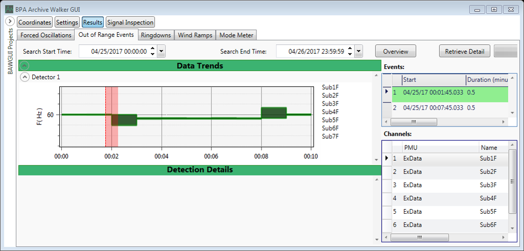 Figure 16: GUI display after loading overview results for the out-of-range detector.
 Figure 17: GUI display after retrieving detailed information about an out-of-range event.
In the Project panel, select the Ringdown task. If this step has not been completed previously, the GUI will produce a dialog box indicating that the example file cannot be found. Navigate to the Data Source tab on the Settings page. In the Example File field, enter the full path to
*\ExampleData\Ringdown\2017\170523\ExData_20170523_000000.csv
The ExampleData folder was included in the download of AW (see Installing and Launching Archive Walker Section). Note that if you navigate to the example file using the GUI, you will need to select JSIS_CSV files in the lower right hand corner of the File Explorer window to see the files. Next, click the Read File button to load the settings and results. Finally, navigate to the Ringdowns tab on the Results page.
The GUI automatically selects the starting time range as the most recent day with an event, in this case May 23, 2017. The upper table lists events, while the lower table lists each of the signals that the event was detected in. In this case, two events were detected. Click the Overview button to load the extrema for the analyzed signals. Once done, the GUI will appear as in Figure 18, with the overview plot to the left. Note that even with this course data, it is clear that the first event is less severe than the second. In the overview plot, the event selected in the upper table is highlighted. To select a different event, simply click it in the table.
To obtain detailed information about the second event, begin by zooming in on it, as in Figure 19. Note that the table of events automatically updates to contain only events within the selected time period. Clicking the Retrieve Detail button reruns the analysis and creates additional plots, as displayed in Figure 19. The top plot in the Detection Details section displays all of the analyzed signals. Below it, thumbnails are provided for each of these signals. Clicking on the thumbnail will display a plot of the signal and a plot of the detector’s operation (see the Ringdown Detector Section). Right-clicking on any of the plots generated by clicking the Retrieve Detail button will provide the option to jump to the Signal Inspection page so that additional signals can be reviewed.
 Figure 18: GUI display after loading overview results for the ringdown detector.
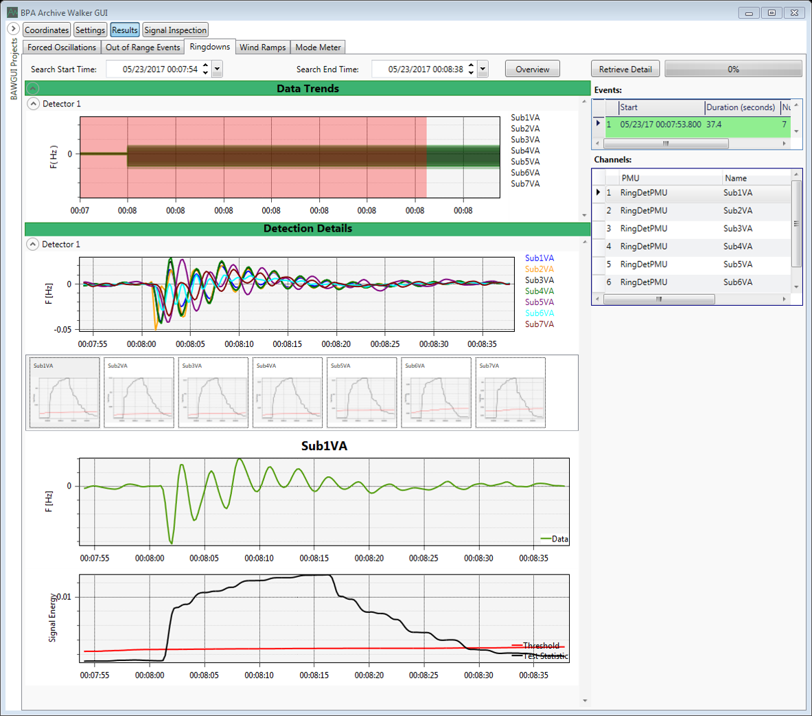 Figure 19: GUI display after retrieving detailed information about a ringdown.
In the Project panel, select the WindRamp task. If this step has not been completed previously, the GUI will produce a dialog box indicating that the example file cannot be found. Navigate to the Data Source tab on the Settings page. In the Example File field, enter the full path to
*\ExampleData\WindRamp\2017\170203\ExData_20170203_000000.csv
The ExampleData folder was included in the download of AW (see the Installing and Launching Archive Walker Section). Note that if you navigate to the example file using the GUI, you will need to select JSIS_CSV files in the lower right hand corner of the File Explorer window to see the files. Next, click the Read File button to load the settings and results. Finally, navigate to the Wind Ramps tab on the Results page.
The GUI automatically selects the starting time range as the most recent day with an event, in this case February 3, 2017. The table lists events active during the selected time range. In this case, two events were detected. Click the Overview button to load the extrema for the analyzed signals. Once done, the GUI will appear as in Figure 20, with the overview plot below the table. In the overview plot, the event selected in the table is highlighted. To select a different event, simply click it in the table.
 Figure 20: GUI display after loading overview results for the wind ramp detector
In the Project panel, select the VoltageStability task. If this step has not been completed previously, the GUI will produce a dialog box indicating that the example file cannot be found. Navigate to the Data Source tab on the Settings page. In the Example File field, enter the full path to
*\ExampleData\VoltageStability\2017\170425\ExData_20170425_000000.csv
The ExampleData folder was included in the download of AW (see the Installing and Launching Archive Walker Section). Note that if you navigate to the example file using the GUI, you will need to select JSIS_CSV files in the lower right hand corner of the File Explorer window to see the files. Next, click the Read File button to load the settings and results. Finally, navigate to the Voltage Stability tab on the Results page.
The GUI automatically selects the starting time range as the most recent day with an event, in this case April 25, 2017. The upper table lists events, while the lower table lists each of the sites that the event was detected in. In this case, nine events were detected. Click the Overview button to load the extrema for the analyzed signals. Once done, the GUI will appear as in Figure 21. Under the Stability Indices banner, the extrema of the stability metrics derived for each of the included Thevenin estimation algorithms are plotted. In the example all five methods are implemented, but in the figure the results from three of them have been collapsed. Under the Out-of-Range Data Trends banner, overview plots from all out-of-range detectors are plotted. The red rectangles that are overlaid indicate detected events. These plots are provided because out-of-range voltage events are useful when considering voltage stability.
To obtain detailed information about the decaying stability, zoom from approximately 00:04:00 to 00:15:59 and set the Prediction Delay field to 30 seconds. Next, click the Retrieve Detail button to rerun the analysis and generate additional plots, as displayed in Figure 22. The plots under the Validation banner include the measured bus voltage and an estimate of the voltage based on the Thevenin equivalent. Good agreement between these values is one indicator that the Thevenin equivalent is a good approximation. Clicking on the thumbnails allows the results from different Thevenin equivalent estimation methods to be reviewed.
 Figure 21: GUI display after loading overview results for the voltage stability detector.
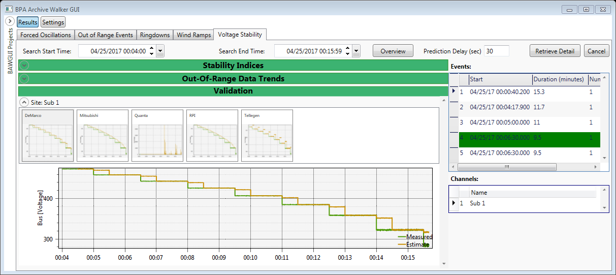 Figure 22: GUI display after retrieving detailed information about the decaying voltage stability.
In the Project panel, select the ModeMeter task. If this step has not been completed previously, the GUI will produce a dialog box indicating that the example file cannot be found. Navigate to the Data Source tab on the Settings page. In the Example File field, enter the full path to
*\ExampleData\ModeMeter\2017\170523\ExData_20170523_000000.csv
The ExampleData folder was included in the download of AW (see the Installing and Launching Archive Walker Section). Note that if you navigate to the example file using the GUI, you will need to select JSIS_CSV files in the lower right hand corner of the File Explorer window to see the files. Next, click the Read File button to load the settings.
As discussed in the Mode Meter Section, the mode meter tool is used to generate data, rather than to detect events. Thus, the output of the mode meter tool is not displayed on the Results page. To see the output of the mode meter example, navigate to the folder
*\Projects\Project_Examples\Task_ModeMeter\Event\MM\Meter1
The Projects folder was included in the download of AW (See the Installing and Launching Archive Walker Section). The folder name Meter1 corresponds to the Mode Meter Name parameter in the setup of the tool. The file 170523.csv contains the results for May 23, 2017. These results are displayed in Figure 23. Column A contains timestamps, columns B through H contain measurements to capture system conditions, and columns I and J contain damping ratio and frequency estimates, respectively. The timestamps specify the time that the mode estimates were generated and the system conditions were collected. For the system condition measurements, row 2 lists the signal names, row 3 contains the signal type, and row 4 specifies the units. For the mode estimates, row 2 contains the name of the mode specified in the Mode of Interest field in the tool’s setup, row 3 specifies the signal used to generate the estimate, and row 4 lists the mode meter algorithm. In this example, system frequency measurements are collected alongside estimates of a system mode near 0.22 Hz.
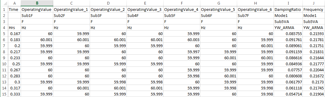 Figure 23: Example output of the mode meter tool contained in 170523.csv.
Archive Walker offers several methods of exporting results as reports or datasets that can be passed to other tools for further analysis. Details are provided in the following subsections.
Data can be exported from the Out-of-Range and Ringdown detectors in much the same way. For data to be exported, detailed detection results must first be retrieved by clicking the Retrieve Detail button on the Out of Range Events or Ringdowns tabs under the Results page. To export the signals analyzed by detectors, click the Export Data botton (highlighted by a blue box in Figure 24). A popup will appear (red box in Figure 24) allowing the user to select which detectors should be included in the export. All signals must have the same sampling rate. After selecting detectors and clicking the Export Data button, a file explorer will appear (green box in Figure 24) allowing the user to specify a name and location for the exported file. Archive Walker automatically appends the start time to the provided file name. The data is exported in JSIS-CSV format.
After the data is exported, a second popup will appear asking if the user would like to update the OBAT preset file (red box in Figure 25). The Oscillation Baselining and Analysis Tool (OBAT) performs small-signal stability analysis by estimating a power system's modes of oscillation. Further information and download instructions for this free tool are available at https://store.pnnl.gov/content/oscillation-baselining-and-analysis-tool-obat. OBAT reads the JSIS-CSV files exported by AW and uses an xml file to store lists of signals in presets and link signals to geographic locations. Archive Walker is able to update this xml file with the locations of signals specified on the Signal Coordinates Setup tab. If desired, it also updates the xml file with a new preset containing the signals in the exported dataset.
If the user selects Yes in the first popup, another window will open (orange box in Figure 25). This window allows the user to specify the name of a new preset containing the exported signals. Clicking the folder button (blue box in Figure 25) opens a file explorer (green box in Figure 25) to locate OBAT's PreSets.xml file, which is stored in the tool's Settings folder. After these steps are completed, the exported data is ready for analysis in OBAT.
 Figure 24: Screen capture during export of event data.
 Figure 25: Screen capture during update of an OBAT preset file.
Mode meter reports can be used to highlight periods where a mode's damping fell below a user-specified threshold. To generate a report, click the Generate Report botton (blue box in Figure 26) from the Mode Meter tab. A popup window (red box in Figure 26) will appear and allow the user to set up the report's parameters. Graphical reports are produced as Microsoft Word documents containing plots of mode frequency, mode damping, and baselining signals for periods of interest. Tabular reports are produced as CSV files listing periods of interest.
 Figure 26: Screen capture of setup of a mode meter report.
The Signal Inspection page can be used to export signals unavailable on results tabs. After signals are plotted, right-click and select the Export Data option (red box in Figure 27). A popup window will appear (green box in Figure 27) allowing the user to specify the location and name for the file. The starting time of the dataset will automatically be appended to the provided name. Data is exported in JSIS-CSV format.
 Figure 27: Screen capture of data export from the Signal Inspection page.
Results and data can be moved for convenience or collaboration between AW users. The processes for handling changes to the location of results and data are distinct and will be described separately.
Moving results is straightforward, but requires a high-level understanding of AW’s storage structure. For the results storage path, projects, and tasks in the example Project panel of Figure 28, AW automatically generates the subfolders in Figure 29. The results of each task are stored in a folder together. These task folders are stored in the folder for their associated project. To transfer results, simply move the folders at any level in Figure 29. Note that if individual tasks are moved, they must be placed under new folders that match the naming convention Project_ProjectName, where ProjectName can be selected by the user. When moving whole project folders, it is best practice to place them in a location occupied only by other AW project folders. If any tasks have signals associated with geographic locations, the SiteCoordinatesConfig.xml file must also be transferred and placed within the main folder containing projects. After relocating the results, simply select the new results storage location in the GUI’s Project panel (see the Project Panel Section). The results can then be viewed from their new location.
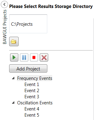 Figure 28: Example Project panel.
 Figure 29: Structure of results storage corresponding to the projects and tasks in Figure 28.
After AW analyzes a set of data, it still relies on the data to produce a detailed review of results (see the Results Hierarchy Section). If the data is moved after a task is saved, the user must specify the new location in the GUI. Each time a task is selected, the GUI determines whether the example file entered on the Data Source tab is available. If it is, it reads the file and populates the Settings page and the Signal Selection panel. If it is not, the GUI requests that the user enter a new example file. When selecting a task after moving the analyzed data, the GUI will make this request. In response, navigate to the Data Source tab under the Settings page. Enter the new path to the example file and click the Read File button. The GUI will update the configuration file for the task and then populate the Settings page and the Signal Selection panel. Once this is done, results can be reviewed as usual.
The main AW tool is accompanied by two tools to enhance functionality. These tools are described in this section.
The Archive Walker Real-Time Display AW-RTD application is intended for use alongside the main AW tool while it is operating in Real-Time mode. It does not impact the setup of an AW analysis or generate results; it simply displays the results produced by AW as they become available.
The installer for AW-RTD can be found within the ArchiveWalkerRealTimeDisplay folder, which is included in the zip file alongside the main ArchiveWalker folder. To install AW-RTD, simply double click the ArchiveWalkerRTD_Installer.exe file. The tool depends on the R2018a (9.4) MATLAB runtime, just as AW does. If AW has already been launched, it should already be installed. During installation, the user may opt to place a shortcut on the desktop. The application can be launched from this shortcut or by navigating to the executable, typically at
C:\Program Files\ArchiveWalkerRTD\application.
A screen capture of the AW-RTD application during setup is provided in Figure 30. To begin, enter the project path described in the Project Panel Section. The Project dropdown will automatically be populated with a list of available projects. When a project is selected, the Task dropdown will automatically be populated with a list of available tasks. The Window dropdown allows the user to select how many minutes of past results should be displayed. After all selections are made, press the Run button to begin displaying results. Note that the main AW tool must be running in Real-Time mode for results to be displayed.
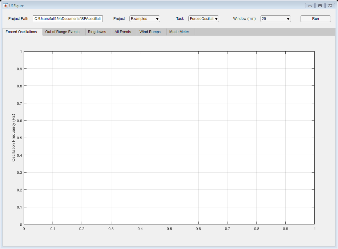 Figure 30: Screen capture of the AW-RTD during setup.
Each detector within AW is designated a tab within the AW-RTD application. An additional All Events tab is included to indicate the occurrence of forced oscillations, out-of-range events, and ringdowns. Each tab is described in the following subsections.
Detected forced oscillations are indicated on the plot with horizontal lines, similar to the plot in Figure 14. Oscillation frequency is plotted along the y-axis and time is plotted along the x-axis. Oscillations with an associated alarm are depicted in red, while non-alarm oscillations are black.
The display of Out-of-Range event detector outputs is similar to the overview plot in Figure 16. The max and minimum of each analyzed signal are plotted, and red rectangles are used to indicate the occurrence of events. The output of multiple detectors can be displayed by selecting the appropriate sub-tab at the top of the window.
The display of Ringdown event detector outputs is similar to the overview plot in Figure 18. The max and minimum of each analyzed signal are plotted, and red rectangles are used to indicate the occurrence of events. The output of multiple detectors can be displayed by selecting the appropriate sub-tab at the top of the window.
The display on this tab captures the outputs of detectors for forced oscillations, out-of-range events, and ringdowns. Forced oscillation events are plotted as described in the [Forced Oscillations Tab Section]. Out-of-range and ringdown events are indicated with colored rectangles to indicate the time that they occurred. Signal trends (maximums and minimums) are not displayed.
The display of Wind Ramp detector outputs is similar to the plot in Figure 20. The max and minimum of each analyzed signal are plotted, and red rectangles are used to indicate the occurrence of ramps. The output of multiple detectors can be displayed by selecting the appropriate sub-tab at the top of the window.
The Mode Meter tab allows for the mode estimates from two mode meters to be displayed. Dropdown boxes at the top of the window are automatically populated to allow the user to select a meter, mode of interest, and algorithm. Once selected, plots of damping ratio and frequency estimates are populated. Alert and alarm thresholds are plotted as horizontal lines at 5% and 3% damping ratio levels for reference. Because forced oscillations and large system disturbances can impact the performance of mode meters, plots similar to those on the All Events tab are included at the bottom of the window. The frequency range is limited to capture forced oscillations near the frequency of the mode of interest.
As discussed in the Database as Source Section, the openHistorian Preset Writer application produces preset files that AW uses to tell it which signals to retrieve from openHistorian. To launch the tool, double click the OpenHistorianReader.exe file located within the openHistorianPresetWriter folder, which is included in the zip file alongside the main ArchiveWalker folder. Alternatively, a shortcut can be added to the desktop by right clicking on the exe file. A screenshot of the application is provided in Figure 30.
To begin, edit the Server Settings fields in the upper left corner of the window. These settings can be retrieved from the openHistorian installation. Once complete, press the Get Metadata button to populate the Signal Selection panel on the right side of the window. Previously created presets are listed in the lower left corner of the window. To add a new one, press the green + button and specify the new preset's name. Add signals to a preset using the Signal Selection panel. If the default units are not correct, they can be updated using the Select Unit by Signal Type section on the left side of the window. Presets are saved together in an xml file. Use the buttons in the lower left corner of the window to load and save this xml. Once saved, the preset xml can be provided to AW.
 Figure 30: Screen capture of the openHistorian Preset Writer application.